
Classification using XGBoost in Log-Odds Space


This article builds upon earlier discussions on XGBoost fundamentals and its regression formulation, and focuses specifically on how XGBoost approaches classification. We will look at what changes, why those changes are necessary, and how to think about tree outputs in a probabilistic setting.
Before diving in, I am assuming you are already familiar with:
Core XGBoost concepts and the optimizations that make it efficient
How gradient boosting extends to classification problems
Log-odds, a foundational idea you may have encountered in logistic regression or boosting-based classifiers
With that groundwork in place, we can now unpack what XGBoost is really doing under the hood when the target variable is not continuous, but categorical.
Disclaimers
XGBoost stands for “Extreme Gradient Boosting,” with “extreme” referring to the numerous optimizations that improve both model performance and speed. However, this article focuses solely on understanding how XGBoost solves classification problems at a fundamental level, without diving deep into optimization techniques.
This guide includes manual calculations to illustrate the concepts. In practice, you’ll use libraries to perform these calculations.
Problem Statement
That said, let’s work with my favourite toy dataset with just one feature CGPA to understand XGBoost classification.
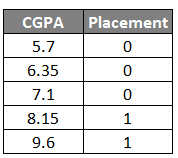
Task is to build an XGBoost classification model that predicts whether a student will get placed based on their CGPA, where 0 = No Placement and 1 = Placement.
XGBoost is essentially Gradient Boosting with specific optimizations. The basic workflow remains the same:
Stage-wise Additive Modeling
Start with a base model
Build multiple small models sequentially
Each model learns from the errors of previous models
Combine all models to create a strong predictor
XGBoost uses a different approach to build decision trees. Instead of using entropy or Gini index, XGBoost uses a metric called Similarity Score.
The Process
Model 1 (Base) → Model 2 (Tree) → Model 3 (Tree) → ... → Final Model
     ↓              ↓                 ↓
  Log Odds    +  η × Tree1    +  η × Tree2  + ...
Where η (eta) is the learning rate, typically set to 0.3.
Stage 1: Base Model (Log Odds)
For classification, we start with log-odds rather than probabilities because probabilities are constrained between 0 and 1 and do not combine linearly during boosting, whereas log-odds allow unrestricted additive updates from multiple trees.
Formula for Log Odds:
Log Odds = log(p / (1 - p))
Where p = probability of positive class (placement = 1)
Calculation:
p = 3/5 = 0.6 (3 students placed out of 5)
Log Odds = log(0.6 / 0.4) = log(1.5) ≈ 0.405
Base Prediction is that all data points start with prediction = 0.405 (in log odds space)
Converting Log Odds to Probability
To calculate errors, we need to convert log odds to probability:
Formula:
Probability = e^(log odds) / (1 + e^(log odds))
Calculation:
Probability = e^0.405 / (1 + e^0.405) ≈ 0.6
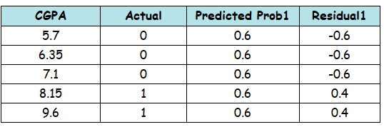
This means our base model predicts 60% probability of placement for everyone, regardless of CGPA.
Calculating Residuals (Pseudo-Residuals)
Residuals = Actual - Predicted
Stage 2: Building the First Decision Tree
Now we build a decision tree using CGPA (input) and Residuals (target).
Step 1: Create Root Node
Place all residuals in a single leaf node: [-0.6, -0.6, -0.6, 0.4, 0.4]
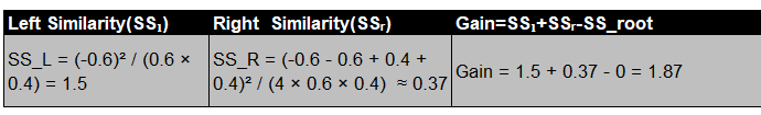
Step 2: Calculate Similarity Score
Formula for Similarity Score(SS) for Classification:
SS = (Σ residuals)² / [Σ(prev_prob × (1 - prev_prob)) + λ]
Where:
Σ residuals = sum of all residuals in the node
prev_prob = previous probability predictions(0.6)
λ = regularization parameter (set to 0 for now)
Similarity Score for Root Node Calculation:
Numerator = (-0.6 - 0.6 - 0.6 + 0.4 + 0.4)² = 0
Denominator = 5 × (0.6 × 0.4) = 1.2
SS_root = 0 / 1.2 = 0
Step 3: Find Best Split
We need to test potential splitting criteria. For consecutive data points, the split point is their average:
Potential Splits:
(5.70 + 6.35) / 2 = 5.975
(6.35 + 7.10) / 2 = 6.725
(7.10 + 8.15) / 2 = 7.625
(8.15 + 9.60) / 2 = 8.875
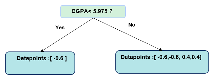
Split 1: CGPA < 5.975
Left Node: [-0.6] Right Node: [-0.6, -0.6, 0.4, 0.4]
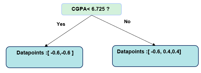
Split 2: CGPA < 6.725
Left Node: [-0.6, -0.6] Right Node: [-0.6, 0.4, 0.4]

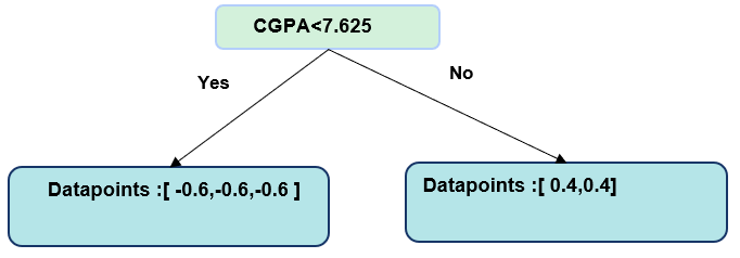
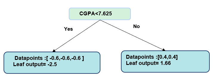
Split 3: CGPA < 7.625
Left Node: [-0.6, -0.6, -0.6] Right Node: [0.4, 0.4]
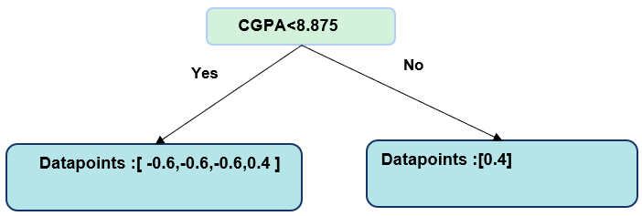
Split 4: CGPA <8.875
Left Node: [-0.6, -0.6, -0.6,0.4] Right Node: [0.4]

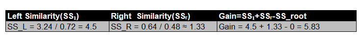
The maximum gain was at split CGPA < 7.625, so this becomes our root node split.
Step 4: Calculate Leaf Output Values
Formula for Leaf Output (Classification):
Output = Σ residuals / [Σ(prev_prob × (1 - prev_prob)) + λ]
Left Leaf (CGPA < 7.625):
Output = (-0.6 - 0.6 - 0.6) / (3 × 0.6 × 0.4)
       = -1.8 / 0.72 ≈ -2.5
Right Leaf (CGPA ≥ 7.625):
Output = (0.4 + 0.4) / (2 × 0.6 × 0.4)
       = 0.8 / 0.48 ≈ 1.66
Stage 2: Making Predictions
Combined Model:
Prediction (log odds) = 0.405 + 0.3 × Tree_output
Where 0.3 is the learning rate (η).
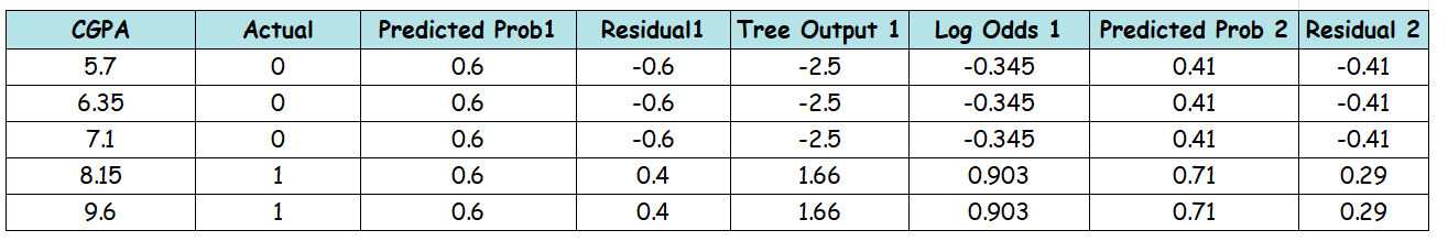
Observation: Errors are reducing! Compare with Stage 1 residuals (-0.6, -0.6, -0.6, 0.4, 0.4).
Stage 3 and Beyond
The process continues in exactly the same way as earlier stages, with each new tree focusing on what the combined model is still getting wrong.
At each stage:
Take the original feature values, such as CGPA, along with the updated residuals from the previous stage.
Train a new decision tree using these residuals as targets. This becomes the next model in the sequence, for example Tree 3.
Scale the output of this tree using the learning rate (η), typically set to 0.3, to control how much it contributes to the overall model.
The model prediction is updated by adding the scaled output of the new tree to the existing prediction:
After updating the prediction:
Convert the accumulated log-odds into probabilities using the sigmoid function.
Compute new residuals based on the difference between the actual labels and the updated probabilities.
Use these new residuals to train the next tree in the sequence.
This cycle repeats for many stages. As more trees are added, the residuals shrink, meaning each new tree makes smaller and more targeted corrections. Eventually, the model reaches a point where additional trees provide minimal improvement, and training stops based on a predefined number of trees or an early stopping criterion.
Prediction on test data (With Example)
Let’s take a test Data with CGPA = 7.0 and Learning rate ( eta = 0.3 )
Step 1: Start with the Base Score
The base probability of 0.6 is converted into log-odds:
Step 2: Pass the Data Point Through the Tree
At inference time, no new trees are built.
The data point is simply passed through Tree 1, where it falls into a specific leaf that produces a log-odds correction.
CGPA = 7.0 falls into the leaf with tree output = −2.5
This tree output represents a log-odds correction.
Step 3: Scale the Tree Output
The tree output is scaled using the learning rate:
Step 4: Accumulate Log-Odds
The scaled correction is added to the base score:
This accumulated value represents the log-odds of the positive class after Tree 1.
Step 5: Convert Log-Odds to Probability
Apply the sigmoid function:
Step 6: Make the Final Classification Decision
Final probability = 0.41
Using a threshold of 0.5, since the predicted probability does not cross the threshold, the model does not have sufficient confidence to predict the positive class and therefore assigns class 0.
Final prediction: Class 0
Loss Function in XGBoost
A loss function in XGBoost measures how far the model’s predictions are from the actual targets. It defines what the model is trying to minimize during training.
For classification, XGBoost predicts values in log-odds space, which are converted into probabilities. The loss function, typically log loss, evaluates how well these probabilities match the true class labels, penalizing confident wrong predictions more than uncertain ones. This is the same loss used in traditional Gradient Boosting.
The difference lies in how the loss is optimized. During training, XGBoost uses both gradients and Hessians of the loss to guide how trees are built, ensuring each new tree makes more precise corrections that reduce the overall loss.
Comparison with Gradient Boosting Classifier
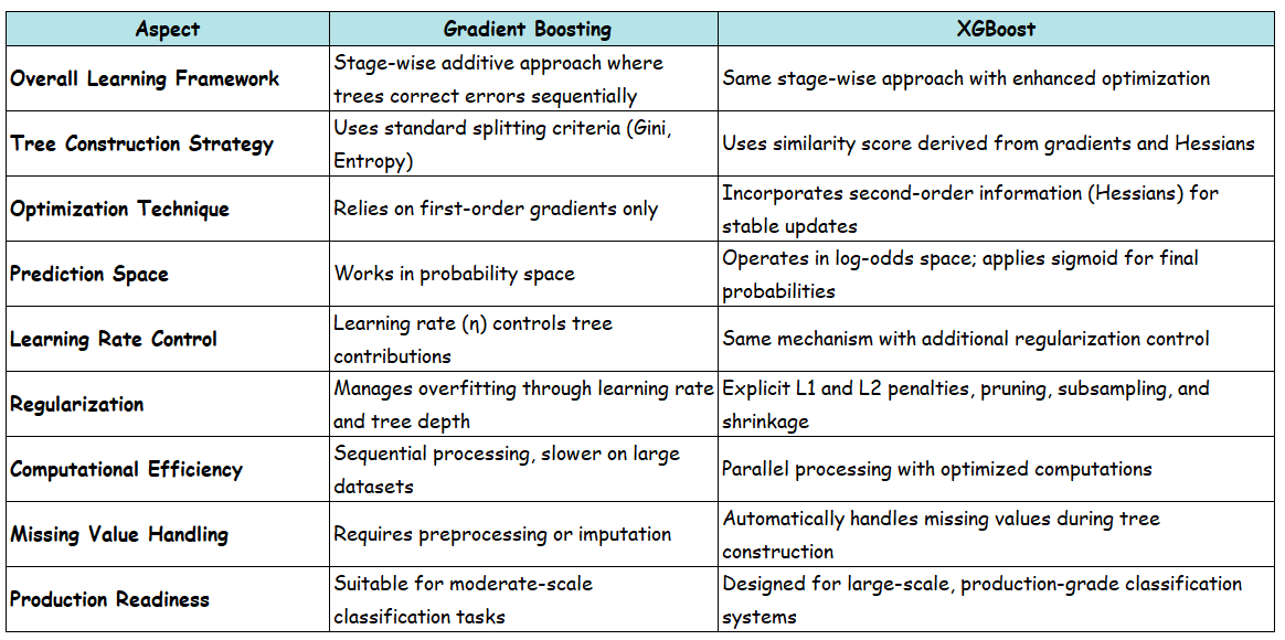
When to Choose XGBoost Over Standard Gradient Boosting
Choose XGBoost when you need production-grade performance, have large datasets, or require built-in regularization and automatic missing value handling. For small datasets where model interpretability is critical, traditional Gradient Boosting may be more appropriate. In most real-world classification tasks, XGBoost’s speed and accuracy advantages make it the default choice.