
DBSCAN(Density-Based Spatial Clustering of Applications with Noise)
A Non-Parametric Approach to Real-World Clustering


DBSCAN represents a paradigm shift in how we approach clustering. Instead of assuming clusters have a particular shape or requiring us to know the number of clusters beforehand, DBSCAN discovers clusters based on density which is a more natural and flexible approach that mirrors how we intuitively understand groupings in the real world.
In this comprehensive guide, let’s explore DBSCAN from the ground up, understanding not just how it works, but why it works, when to use it and how to apply it effectively to real-world problems.
Before we dive deep into DBSCAN, it’s crucial to understand why we need an alternative to K-Means in the first place. K-Means is fast, easy to implement and works well for many datasets. However, it has three fundamental limitations that make it unsuitable for many real-world clustering tasks.
Limitation 1: The Curse of Predefined Clusters
K-Means requires specifying k (the number of clusters) upfront, which introduces several issues:
Uncertain true k: Even domain experts often can’t determine the natural number of clusters without extensive trial and error.
Ambiguous heuristics: Methods like the elbow or silhouette often give unclear or conflicting results.
Dynamic data: Real-world clusters can shift over time, making a fixed k obsolete.
High exploration cost: Finding the optimal k requires multiple runs, increasing computational expense for large datasets.
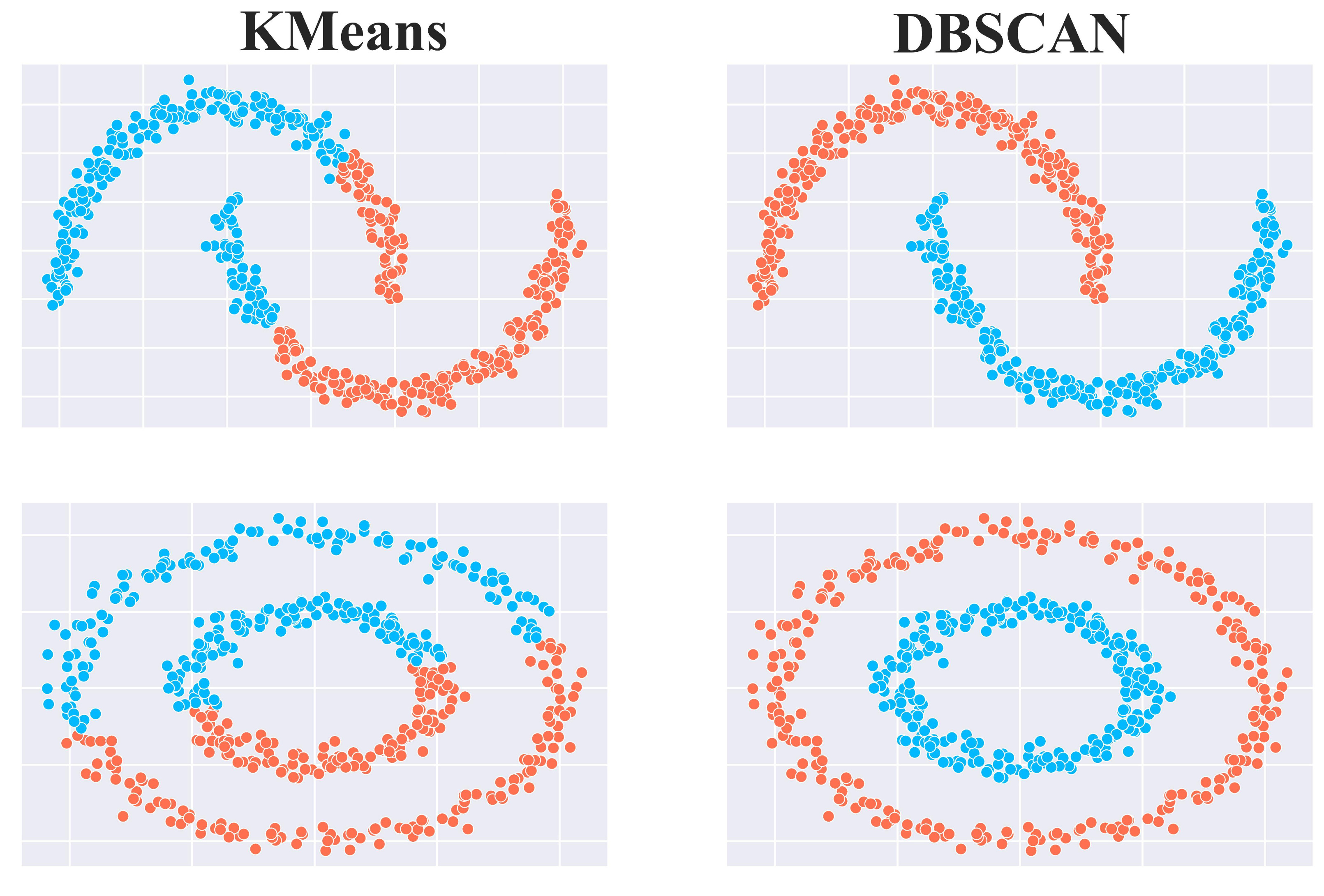
Limitation 2: The Circular Cluster Constraint
K-Means assumes clusters are spherical because it assigns points to the nearest centroid, forming convex, circular (in 2D) Voronoi regions.
Real world Implications:
K-Means often splits or merges elongated or non-convex clusters incorrectly.
K-Means fragments concentric or irregular patterns into circular parts.
Many real-world clusters lack a true center, as they are defined by density or boundaries rather than proximity to a centroid
In short, K-Means fails to capture elongated, curved or arbitrarily shaped clusters due to its circular bias.
Limitation 3: Vulnerability to Outliers
K-Means handles outliers poorly because centroids are mean-based, making them sensitive to extreme values. Outliers can pull centroids away from true cluster centers, distort boundaries, reassign points incorrectly, and even cause the algorithm to form separate clusters for isolated outliers, leading to unstable and inefficient clustering.
For example when clustering income data (mostly $30K–$150K) with a few billionaires, K-Means gets distorted ,it either drags the centroid upward, merging upper-middle-class earners with billionaires or wastes a cluster on just a few outliers. Since K-Means lacks outlier detection, every point is forced into some cluster, even if it doesn’t fit naturally.
The Need for a Better Solution
K-Means’ core flaws i.e fixed cluster count, circular shape bias and outlier sensitivity limit its real-world use. We need an algorithm that automatically finds clusters, handles arbitrary shapes and treats outliers as noise.This is exactly what DBSCAN does.
The Core Philosophy: Density Over Distance
DBSCAN redefines clustering by focusing on density instead of distance. Rather than finding the nearest center (as in K-Means), it asks whether a point lies in a dense or sparse region,very much like crowds in a plaza, cities amid countryside or star clusters in space. It mathematically formalizes this intuitive idea.
DBSCAN works by:
Identifying dense regions(many points in a small area) in the data space
Treating these dense regions as clusters
Recognizing sparse regions(few points spread out) as boundaries between clusters or as noise
To implement density-based clustering, we need a way to measure density around any given point. DBSCAN does this with just two parameters.
The Two Key Parameters
1. Epsilon (ε)
Defines the radius of the neighborhood around a given data point
Represents the maximum distance between two points for them to be considered part of the same neighborhood
Think of it as drawing a circle (or sphere in higher dimensions) around each point
2. MinPts (Minimum Points)
Specifies the minimum number of points required to form a dense region
This threshold determines whether an area is considered dense or sparse
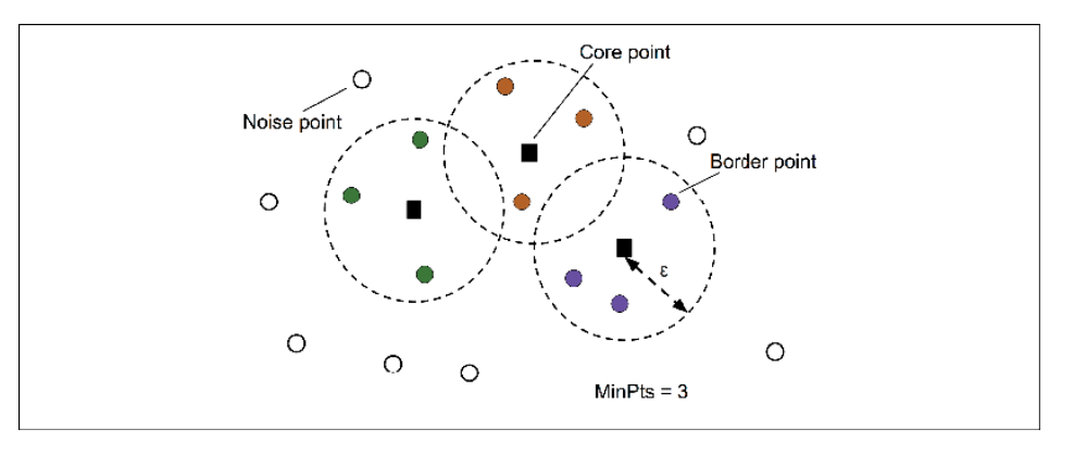
Example: Imagine drawing a circle with radius ε = 1 unit around a point. If you decide MinPts = 4 and there are 7 points within that circle, the area around that point is considered dense. If there are only 2 points, it’s sparse.

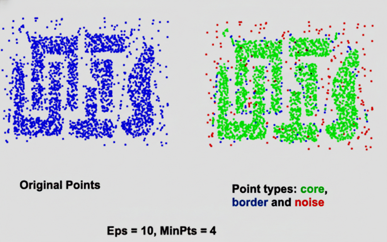
How DBSCAN Sees Your Data: Core, Border, and Noise Points
To understand how DBSCAN forms clusters, it’s essential to see how it categorizes data points based on local density. Every point in the dataset is classified into one of three types: core points, border points or noise points.

1. Core Points
A point is a core point if it has at least MinPts points (including itself) within its ε-neighborhood. If you draw a circle of radius ε around a point and find at least MinPts points inside that circle, it becomes a core point. In the diagram, blue squares🟦 represent core points inside the ε-neighborhood.
Visually, core points form the dense “body” of each cluster, usually shown in the cluster’s main color. They’re crucial because they define the cluster’s shape and location even without border points, the cluster’s structure remains visible.
2. Border Points
A border point must satisfy two conditions:
It is NOT a core point (has fewer than MinPts within its ε-neighborhood)
It is within ε distance of at least one core point (lies on the edge of a cluster)
In the diagram, black circles ⚫ represent border points.
They lie close enough to dense regions to be part of a cluster but are not dense enough themselves to be core points.Border points form the cluster’s “outer shell,” marking the transition between dense and sparse regions.
3. Noise Points
A noise point is neither a core point nor a border point(shown as white circles ⚪in the diagram).
Noise points are isolated outliers in sparse regions, far from any cluster. Unlike K-Means, DBSCAN leaves them unassigned. They represent rare, anomalous or even valid but unusual data such as rare events, transition states or data errors.
The image below illustrates how DBSCAN classifies data points based on local density.
Essential Concepts to Grasp Before Diving Into DBSCAN
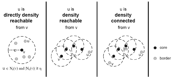
1. Direct Density Reachability
In the first diagram, u is directly density-reachable from v because:
u lies within v’s ε-neighborhood (inside the dashed circle), and
v is a core point (shown as a filled black circle).
This relationship represents the most basic form of reachability .A direct link from one core point to another nearby point within distance ε.
2. Density Reachability
In the second diagram, u is density-reachable from v through a chain of core points.
Even if u is not directly within v’s ε-neighborhood, it can be reached by moving from one core point’s ε-neighborhood to another’s.
This is how DBSCAN expands clusters by connecting points through overlapping ε-neighborhoods of core points.
3. Density Connectivity
In the third diagram, u and v are density-connected because both are density-reachable from a common core point m.
This means that even if u and v cannot reach each other directly, they belong to the same cluster through their connection to m.
This figure illustrates how DBSCAN links points based on density, expanding clusters through direct reachability, chaining via core points and finally connecting separate chains into unified clusters.
The DBSCAN Algorithm: Step by Step
Step 0: Choose Parameters
Select the two key parameters:
ε (epsilon): The neighborhood radius.
MinPts: The minimum number of points required to form a dense region.
Step 1: Classify All Points
Using ε and MinPts, label every point as one of the following:
Core Point: Has at least MinPts points (including itself) in its ε-neighborhood.
Border Point: Lies within the ε-neighborhood of a core point but has fewer than MinPts itself.
Noise Point: Neither a core nor a border point.
Step 2: Form Clusters from Core Points
Start with any unclustered core point — This point becomes the seed of a new cluster.
Expand the cluster.
Find all points within its ε-neighborhood.
Add these points to the cluster.
For every new core point added, repeat the process , include all points that are directly density-reachable or density-connected.
Continue expansion until no new points can be added.The cluster grows outward through chains of connected core points.
Move to the next unclustered core point.If it’s not density-connected to any existing cluster, it becomes the starting point of a new cluster.
Step 3: Assign Border Points
Assign each unclustered border point to the cluster of its nearest core point.
Step 4: Leave Noise Points Unassigned
Any remaining points that are neither core nor border are marked as noise .These are true outliers that don’t belong to any cluster.
DBSCAN in Practice: Using scikit-learn
In scikit-learn, DBSCAN has two main parameters:
1. eps (epsilon):
Larger epsilon → bigger neighborhoods → larger clusters, more density connections
Smaller epsilon → smaller neighborhoods → more smaller clusters
2. min_samples (MinPts):
Increasing min_samples: Requires more points to form a dense region, resulting in fewer, tighter clusters. More points may be classified as noise.
Decreasing min_samples: Makes it easier to form dense regions, resulting in more clusters with looser boundaries. Fewer points are classified as noise.
Effect of different values of epsilon and min_samples
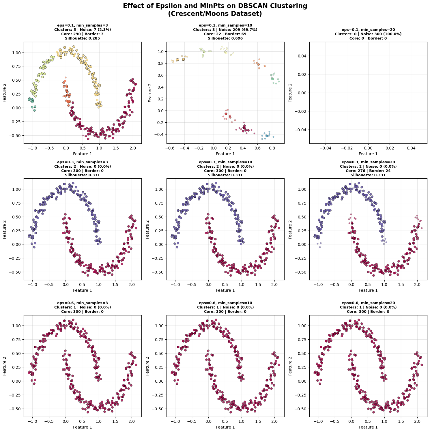
The diagram visually demonstrates how ε (epsilon) and MinPts interact to shape DBSCAN’s clustering results:
As ε increases, neighborhoods grow larger clusters begin to merge, reducing the total number of clusters and noise points.
As MinPts increases, the density requirement becomes stricter fewer points qualify as core, leading to more noise and fewer clusters.
Small ε + Small MinPts means many small, fragmented clusters.
Small ε + Large MinPts means mostly noise (too strict).
Large ε + Small MinPts means few large, merged clusters.
For the above dataset the sweet spot (medium ε ≈ 0.3, MinPts = 3–10) forms well-defined, separate clusters that match the structure of crescent-shaped data.
Why DBSCAN Excels and Its Key Advantages and Disadvantages
DBSCAN’s Strength lies in handling complex shapes.Unlike K-Means, which depends on centroids and distance to neighbors, DBSCAN relies solely on data density. This enables it to detect clusters of any shape, including:
Concentric circles
Elongated or curved clusters
Irregular or non-convex boundaries
Here a quick comparison between K-Means and DBSCAN
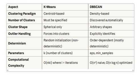
Advantages of DBSCAN
Robust to Outliers: Explicitly identifies and separates noise points from clusters.
No Need to Predefine Cluster Count: Automatically determines how many clusters exist.
Handles Arbitrary-Shaped Clusters: Can find clusters of any form, driven by density rather than distance to a center.
Simple to Tune: Requires only two parameters—ε (epsilon) and MinPts.
Disadvantages of DBSCAN
Sensitivity to Hyperparameters: Small changes in epsilon can produce significantly different results
Difficulty with Varying Density Clusters: If one cluster is very dense and another is less dense, DBSCAN struggles because it uses the same epsilon and MinPts values for all clusters
No Direct Prediction: To cluster new data points, you must retrain on the entire dataset to reestablish density connections.
Poor Performance in High Dimensions: In high-dimensional spaces, distances become less meaningful (curse of dimensionality). Dimension reduction techniques like PCA should be applied before clustering
Evaluation and Parameter Selection
Since DBSCAN doesn’t need a predefined number of clusters, we evaluate its results using metrics that measure cluster cohesion and separation.
1. Silhouette Score
Measures how well each point fits within its cluster.
\(s(i) = \frac{b(i) - a(i)}{\max(a(i), b(i))}\)a(i) = average distance from i to other points in the same cluster
b(i) = average distance from i to points in the nearest different cluster
It ranges between +1 which means well-clustered and -1 which means misclassified and 0 means boundary .Higher average scores (excluding noise) indicate better clustering.
2. Davies–Bouldin Index (DBI)
Measures average similarity between clusters.
Lower values means better separation.
\(DB = \frac{1}{k} \sum \max(R_{ij})\)
Where R_ij is the similarity between clusters i and j based on within-cluster distances and between-cluster separation.
3. Calinski–Harabasz Index (CH)
Ratio of between-cluster to within-cluster variance.
Higher values means clearer, more distinct clusters.
\(CH = \left( \frac{\text{trace}(B_k)}{\text{trace}(W_k)} \right) \times \left( \frac{n - k}{k - 1} \right)\)B_k = between-cluster dispersion matrix
W_k = within-cluster dispersion matrix
n = number of points
k = number of clusters
Use these metrics to compare different ε and MinPts values when tuning DBSCAN for best results. DBSCAN can be aggressive in classifying points as noise and is very sensitive to parameters, but it excels at identifying outliers which is a significant advantage over K-Means.
Real-World Applications of DBSCAN
1. Spatial Data Analysis
Particularly well-suited for geographic data, DBSCAN identifies regions of similar land use in satellite images or groups locations with similar activities in GIS (Geographic Information Systems).
2. Anomaly Detection
The algorithm’s ability to distinguish noise from core clusters makes it invaluable for detecting fraudulent banking transactions or identifying unusual patterns in network traffic.
3. Image Processing
Used for object recognition and image segmentation, grouping pixels or features that form meaningful structures.
4. Bioinformatics
Identifies groups of genes with similar expression patterns in gene expression data analysis, indicating potential functional relationships.
5. Customer Segmentation
In marketing and business analytics, DBSCAN clusters customers with similar buying behaviors or preferences.
6. Astronomy
Employed for star cluster identification, grouping stars based on physical proximity or other attributes.
7. Environmental Studies
Clusters areas based on pollution levels or identifies regions with similar environmental characteristics.
8. Traffic Analysis
Identifies hotspots of traffic congestion or clusters routes with similar traffic patterns in transportation studies.
9. Machine Learning and Data Mining
Used for exploratory data analysis, uncovering natural structures or patterns in data that might not be apparent otherwise.
10. Social Network Analysis
Detects communities or groups within social networks based on interaction patterns or shared interests.