
Dropout, Batch Normalization, and Regularization in Deep Neural Networks

You’ve built a neural network. You’ve fed it data for hours. Training accuracy? Sky high. Validation accuracy? Barely moving.
This gap is called overfitting. But it is not the only wall people hit when moving from toy examples to real-world problems. Training can also become slow, unstable, and extremely sensitive to things like your learning rate, weight initialization, and network depth.
The good news is that it is a solvable problem. The toolkit has three items: Batch Normalization, Dropout, and Regularization. Together they tackle unstable training and poor generalization.
By the end of this article, you will know exactly what each one does, why it works, and when to use it.
Batch Normalization
The Problem Batch Normalization Solves: Internal Covariate Shift in Deep Networks
Why We Normalize Inputs in the First Place?
Say you are training a neural network on student data, with two input features: CGPA (ranges from 0 to 10) and IQ (ranges from 0 to 150). These two features live on completely different scales. One is in single digits. The other goes up to the hundreds.
When you pass unnormalized data into a neural network and plot the cost function’s contour, it looks like a stretched oval tilted at an angle. It is much wider in one direction than the other. Wide in the IQ direction, narrow in the CGPA direction, because the IQ values dominate with their larger magnitude.
This elongation creates a serious problem for gradient descent. If you set a high learning rate, gradient descent overshoots in the wide direction. It bounces back and forth, never settling. So you are forced to keep the learning rate low. And with a low learning rate, you take tiny steps. Training becomes slow, and sometimes unstable.
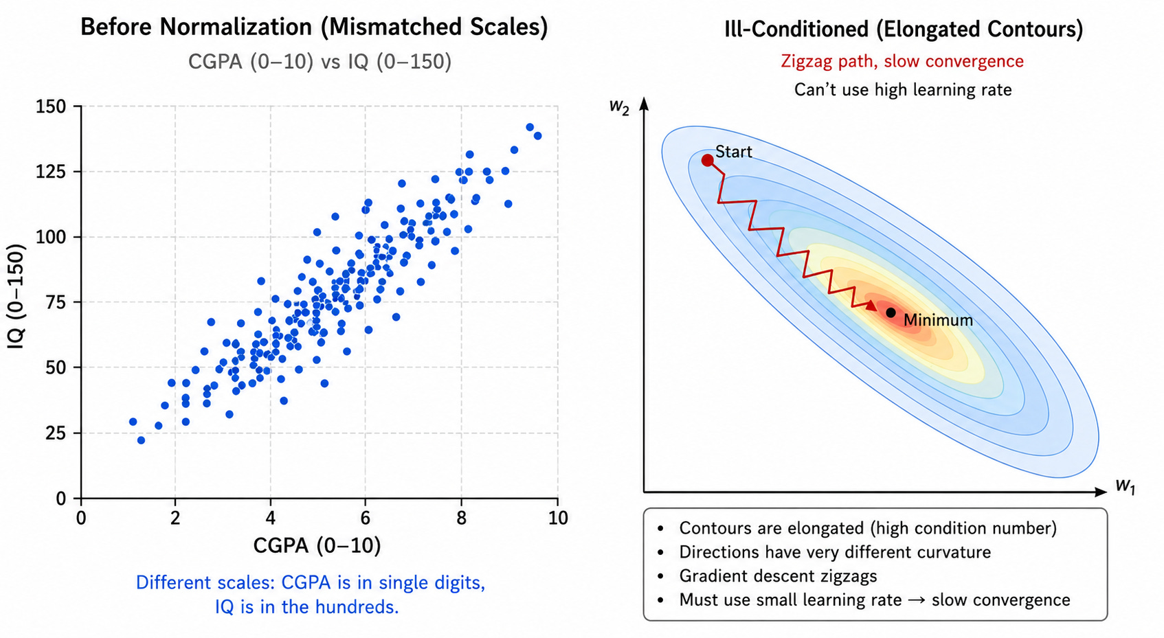
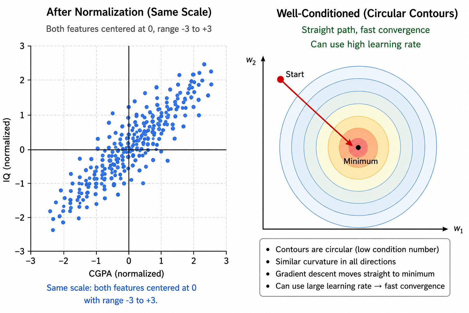
When you normalize your inputs so that each feature has mean = 0 and standard deviation = 1, the loss function’s contour becomes circular and uniform in every direction. Gradient descent can now use a much larger learning rate, take confident steps in any direction, and reach the minimum quickly from many different starting points.
x_norm = (x - μ) / σ
μ = mean of the feature across the training set
σ = standard deviation of the feature
After normalization, your data looks like a tidy cluster centered at 0. The features are on the same scale. Gradient descent has a smooth, uniform bowl to roll down into.
That is the input side.
Here is what happens once the data is inside the network.
Internal Covariate Shift
Normalization gives the network a clean start. But as data travels through layer after layer, the outputs of each layer become the inputs to the next. Every layer feeds the one after it.
And here is the problem. Every time the weights in layer 1 update during backpropagation, the distribution of its outputs shifts. Layer 2 now receives inputs with a different distribution than before. It adjusts its weights accordingly, but that adjustment shifts its own outputs. So layer 3 is now chasing a different distribution too. And this cascades all the way through.
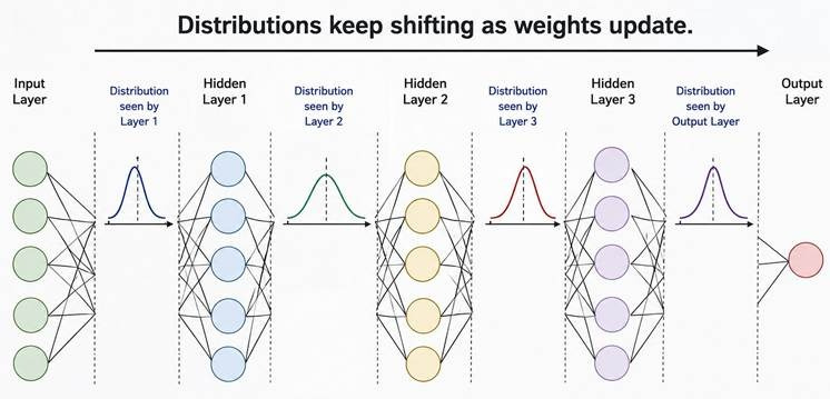
This cascading instability is called Internal Covariate Shift. It is the change in the distribution of network activations due to the change in parameters during training.
The word internal distinguishes this from the regular covariate shift.
The Covariate Shift
Before we get to the internal version, let us understand regular covariate shift. Imagine you train a model to classify roses versus other flowers. During training, every rose image you provide is a red rose. Your model learns to distinguish roses from other flowers, but it heavily associates “rose” with the red color.
Now during testing, you show it white roses, pink roses, yellow roses. The relationship between the input (rose) and output (label: rose) is still the same. But the distribution of the input images has shifted. The model struggles not because the underlying truth changed, but because the data looks different from what it was trained on. This is Covariate Shift. Same relationship, different distribution.
Internal Covariate Shift is the same problem, but happening inside the network between its own layers, on every single training step.
Every hidden layer is like a small sub-network. Its inputs are the outputs of the previous layer. And those outputs keep changing their distribution as the earlier weights update. So every hidden layer is constantly trying to learn from a moving target.
The Telephone Game is a perfect everyday analogy for this. The first child is told “peace.” They whisper it to the next child, who hears “peas.” That child whispers “niece.” The next one passes on “cheese.” The last child hears “please.”
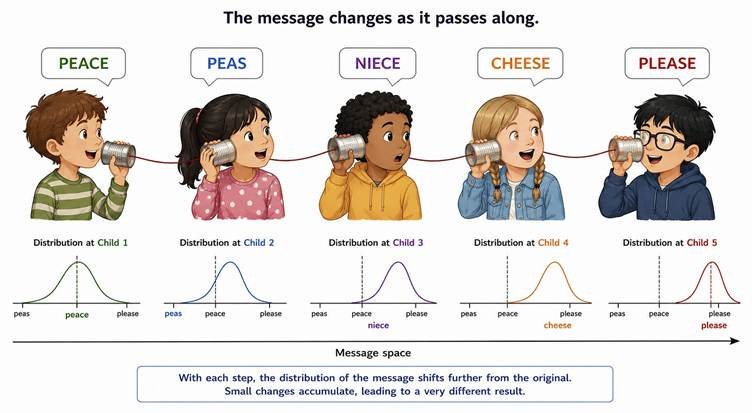
Nobody intentionally changed the message. But each person interpreted what they heard slightly differently and passed it on. By the end, the information has drifted far from the original.
The same thing happens inside a deep neural network. Information enters as something meaningful. Each layer transforms it, and because the weights are constantly updating, each layer’s output distribution drifts. By the time you reach the final layers, the signal they receive is quite different from what was originally fed in.
Here is what that instability actually causes:
Gradients become unreliable. Each gradient is computed on the current distribution of inputs. But by the next batch, that distribution has shifted. So the gradient is giving you directions based on a landscape that no longer exists. With a high learning rate, you take a big step in that direction, only to find the target has moved. The next gradient tries to correct, but the distribution has shifted again. Training oscillates and never settles. A low learning rate limits the damage, but it does not fix the root cause.
Poor weight initialization can break training entirely. A large starting weight leads to exploding gradients, where the error signal explodes as it passes backward through the network. On its own, that is already a problem. But combined with shifting distributions, it is worse. The gradients are not just large, they are being computed on a landscape that keeps changing. The network has no stable ground to recover from, and training collapses.
Training slows down the deeper your network gets. Each layer takes the output of the previous layer as its input. If layer 1’s distribution shifts slightly, layer 2 inherits that shift and adds its own on top. Layer 3 inherits both. By layer 10, the signal has been distorted nine times over. The optimizer has to constantly undo the damage from previous steps rather than making clean forward progress. Two steps forward, one step back, repeatedly. The deeper the network, the more this compounds, and the slower training gets.
How Batch Normalization Solves Internal Covariate Shift
Training does not process all data at once. It works in small chunks called mini-batches, typically 32 or 64 data points at a time.
Batch Normalization solves Internal Covariate Shift by applying the same normalization we do to inputs, but this time to the activations of each hidden layer. After each hidden layer computes its activations, we normalize them to have mean = 0 and standard deviation = 1, using statistics from the current mini-batch. That is where the word “batch” comes from.
This way, regardless of how the weights in earlier layers have shifted, each subsequent layer always receives inputs from a consistent, normalized distribution. The moving target problem is solved.
Two important things to note: Batch Norm is applied layer by layer, and it is optional per layer. You can apply it to all hidden layers, or just some. It is not all-or-nothing.
Step-by-Step: How It Works on One Layer
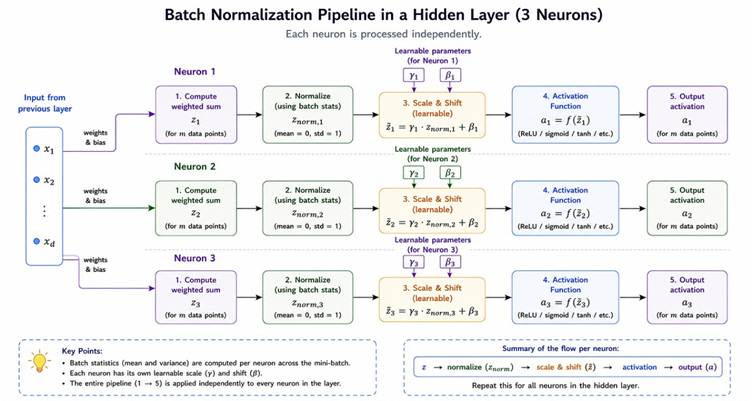
Let’s understand Batch Norm with an example. Say we have a hidden layer with 2 neurons, and we are using a mini-batch of 4 data points. Our data contains student records: CGPA and IQ. We want to predict placement outcome.
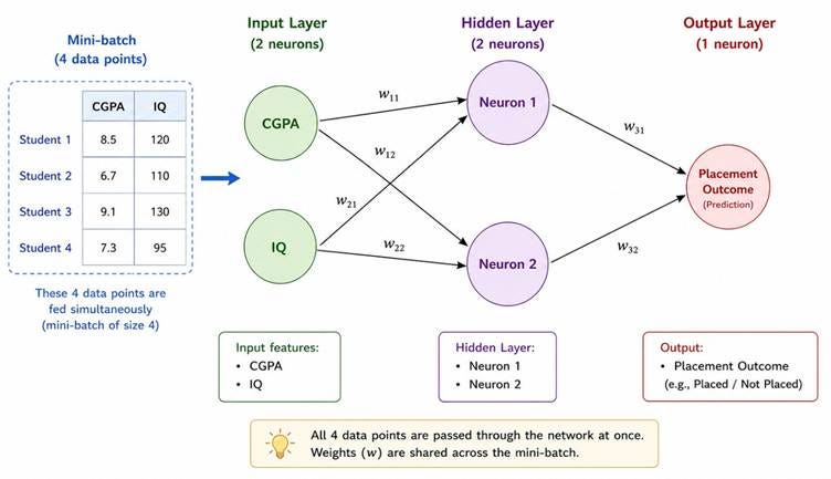
Step 1 — Compute the weighted sum (z)
Each neuron begins by computing its weighted sum for every data point in the mini-batch, where x1 = CGPA and x2 = IQ:
z11 = w11·x11 + w21·x21 + b
z12 = w11·x12 + w21·x22 + b
Because we are sending 4 data points at once, each neuron produces 4 z values, one per data point. So at this stage, we have:
Neuron 1: [z11, z12, z13, z14], one z value for each of the 4 data points
Neuron 2: [z21, z22, z23, z24], its own separate 4 z values
👉 Each neuron is treated completely independently in all subsequent steps. Neuron 1 never shares statistics with Neuron 2.
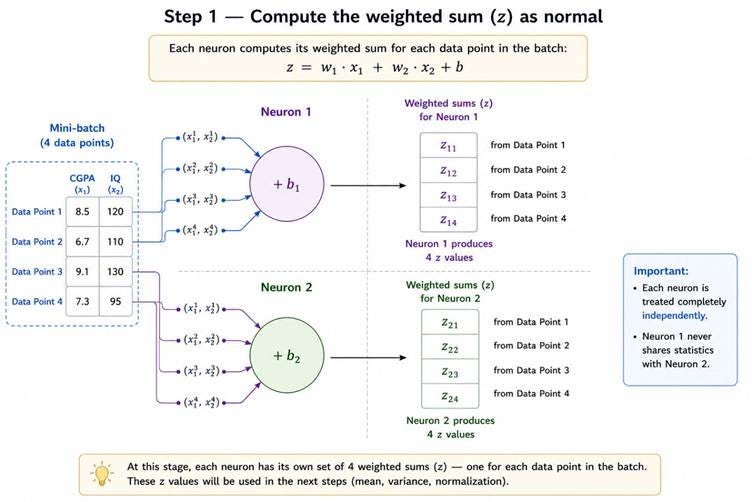
Step 2 — Normalize using batch statistics
For each neuron separately, we now compute the mean and variance across its 4 z values:
μ_B = (1/m) × Σ(z_i) ← mean of the batch
σ²_B = (1/m) × Σ(z_i - μ_B)² ← variance of the batch
Where m = batch size (4 in our example). Here, m = 4, so μ_B is just the average of the 4 z values for that neuron.
Once we have the mean and variance, we normalize each z value:
z_norm_i = (z_i − μ_B) / √(σ²_B + ε)
The ε (epsilon) in the denominator is a tiny number (e.g. 1e-5) added to prevent division by 0 in case the variance is exactly 0. After this step, the 4 normalized values for each neuron have mean = 0 and standard deviation = 1.
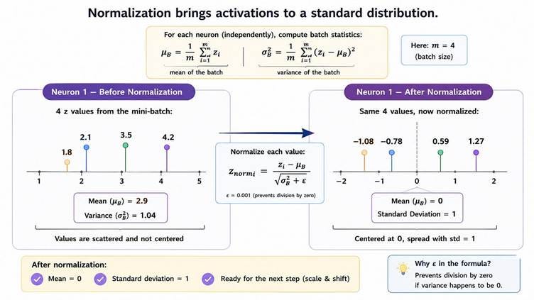
Neuron 1 computes its own μ_B and σ_B from its own 4 z values. Neuron 2 computes its own separate μ_B and σ_B.
Step 3 — Scale and Shift using learnable parameters γ and β
Here is where Batch Normalization becomes truly flexible. After normalizing, we apply one more transformation:
ž_i = γ × z_norm_i + β
Where γ (gamma) is a learnable scale parameter and β (beta) is a learnable shift parameter. These are trained by backpropagation, just like the weights. Every neuron has its own individual gamma and beta.
Why do this after normalizing? It seems counterintuitive. You just brought everything to mean = 0, std = 1, and now you are scaling and shifting it again.
The reason is that normalization always forces a specific distribution. But sometimes the network does not want that. Maybe for a particular layer, the best distribution to work with has a mean of 2 and a std of 3. The network should be free to choose. γ and β give it that freedom.
If normalization turns out to be exactly right, the network will learn γ = 1 and β = 0, and nothing changes from the normalized values. If a different distribution works better, γ and β will shift to produce it.
γ is initialized to 1 and β to 0 at the start of training. During training, backpropagation updates them just like any weight.
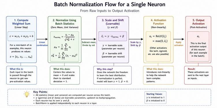
Step 4 — Pass ž through the activation function
The scaled and shifted value ž is finally passed into the activation function (ReLU, sigmoid, tanh, etc.) to produce the neuron’s activation:
a = activation_function(ž)
So the complete sequence for a neuron in a Batch Norm layer is:
z → normalize(z_norm) → scale & shift (ž) → activation function → output → activation a
This entire process repeats for every neuron in the layer. If the layer has 128 neurons, the whole thing happens 128 times independently, neuron by neuron.
Batch Normalization On Test Data
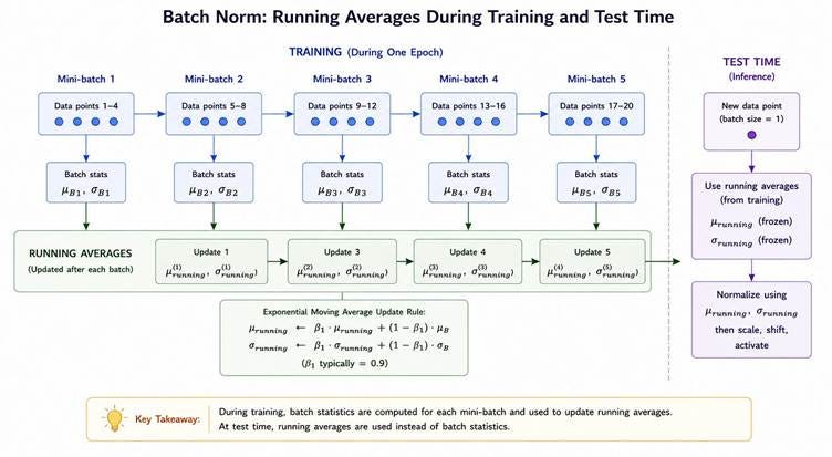
During training, the batch statistics (mean and standard deviation) are computed fresh from each mini-batch. If your batch size is 32, it is the average of 32 values. This works well during training.
But the problem is when you deploy your model, you are often making predictions one data point at a time. Maybe a single student submits their CGPA and IQ and asks for a placement prediction. You cannot compute a mean from one value. The batch normalization formula won’t work, so where do μ_B and σ_B come from?
The solution is to maintain running averages during training and use them during testing.
Say your dataset has 100 students and your batch size is 4. That means your training algorithm runs 25 times per epoch (25 batches). After each batch, you compute μ_B and σ_B for that batch. At the same time, you update a running average that accumulates estimates across all batches seen so far.
μ_running ← β₁ × μ_running + (1 − β₁) × μ_B
σ_running ← β₁ × σ_running + (1 − β₁) × σ_B
The β₁ here (typically 0.9) is the decay rate for the moving average. It gives more weight to recent batches while still keeping a memory of earlier ones. This is the same exponentially weighted moving average idea used in optimizers like Adam.
After 25 batches, you have 25 different estimates of μ_B and σ_B. The running average blends all of them into single stable estimates, which are frozen after training and used during testing.
The 4 Parameters per Neuron
Every neuron in a Batch Norm layer carries 4 associated values:
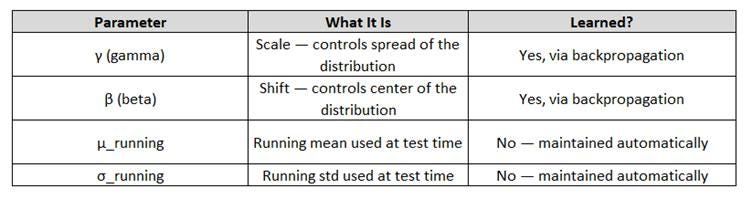
For example, If your hidden layer has 3 neurons and you apply Batch Norm, you add 12 total parameters: 6 learnable (γ and β for each neuron) and 6 non-learnable (running mean and std dev for each neuron).
The Benefits of Batch Normalization
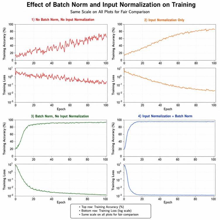
1. Training becomes faster Because each layer receives inputs from a stable, consistent distribution, the optimizer is not fighting against constantly shifting baselines. You can also use a higher learning rate without destabilizing training. Higher learning rate means larger steps, which means faster convergence. In practice, models with Batch Norm often converge in fewer epochs than models without it.
2. Training becomes more stable The cost function landscape becomes more uniform in all directions. Gradient descent can navigate it cleanly from many different starting points, and your hyperparameter choices work over a much wider range of values. You are less likely to accidentally break training by picking slightly wrong hyperparameters.
3. A mild regularization effect (useful side effect) Because μ_B and σ_B are computed from mini-batches rather than the full dataset, there is slight randomness in the normalization at every step. The exact mean and standard deviation change slightly each batch, introducing a small amount of noise into the activations. This acts like a weak regularizer and slightly reduces overfitting. This is a side effect, not the main purpose. You will still need Dropout for serious regularization.
4. Less sensitivity to weight initialization Without Batch Norm, a badly initialized weight can trigger exploding gradients and destabilize training for many epochs. With Batch Norm, the smoother cost function landscape means the optimizer can find its way to a good solution from a much wider range of starting points.
Batch Normalization: Keras Implementation
In Keras, adding Batch Normalization is a single line after each layer you want to normalize:
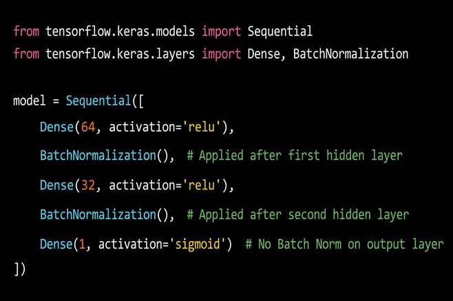
Keras automatically handles the running averages used during testing.
Dropout
The Problem Dropout Solves: Overfitting in Dense Networks
Batch Normalization is primarily about training stability. Dropout is primarily about generalization.
When a neural network overfits, something specific happens inside it. Because the neurons train together on the same data repeatedly, they develop tight dependencies on each other. Neuron A learns to always fire when Neuron B fires. Neuron C learns to correct Neuron A’s errors. Over time, the neurons form a co-dependent committee that only works when all members are present.
This is called co-adaptation. It is the neural network equivalent of a team that has worked together so long that they can only function as a unit. When you show this team new data they have not memorized together, the co-adaptations do not hold and generalization breaks down.
What Dropout Does
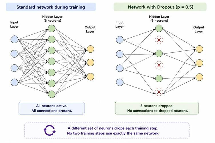
During each training step, every neuron in a Dropout layer is randomly switched off with probability p. Here p is called the dropout rate. A value of 0.5 means half the neurons are switched off each step. A value of 0.2 means only 20% are dropped. Higher p means stronger regularization but more information lost per step. Lower p is gentler but provides weaker regularization.
When a neuron is switched off:
• Its output is set to 0 for that training step
• It does not contribute to the forward pass
• It receives no gradient update during backpropagation
More importantly, a different random set of neurons is dropped each step. So on step 1, neurons 3, 7, and 12 might be off. On step 2, neurons 1, 5, and 9 might be off. No two training steps use exactly the same network.
Why This Forces Better Generalization
When neurons know that any of their neighbors might be randomly absent at any training step, they cannot rely on those neighbors. A neuron that has learned “I just wait for Neuron B to fire and then I amplify it” will be useless during the many steps when Neuron B is switched off.
Instead, each neuron must learn to be useful independently. It has to build its own representation of the data, not just piggyback on others.The result is neurons that stand on their own, and a network that generalizes.
The Ensemble Interpretation
Each training step activates a different random subset of neurons, effectively training a slightly different subnetwork each time. This is called an implicit ensemble. In machine learning, an ensemble means training multiple different models and averaging their predictions. It almost always generalizes better than a single model. Dropout builds this in automatically. During testing, all neurons are active, averaging across all those subnetworks at once. You get the generalization benefit without the cost.
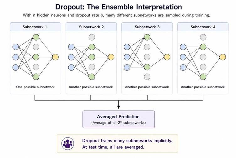
During testing, since all neurons are switched on, to compensate for the fact that more neurons are now active than during training, all weights are scaled down by a factor of (1 - p). Keras handles this automatically in training and test modes.
Dropout Regression Example
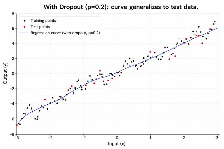
Let’s say we train a neural network on some regression data with a near-linear relationship between input and output. The architecture is simple: 1 input, 2 hidden layers with 128 neurons each (ReLU activation), 1 output neuron (linear activation). Optimizer: Adam. Loss: MSE.
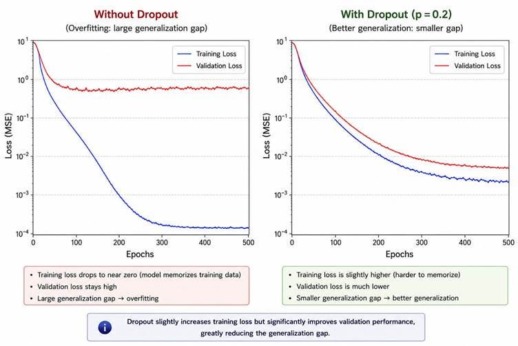
We train for 500 epochs. The results:

When we plot the regression curve without dropout, it hugs every training point tightly. It memorizes the noise. The curve doesn’t fit the test points shown in red.
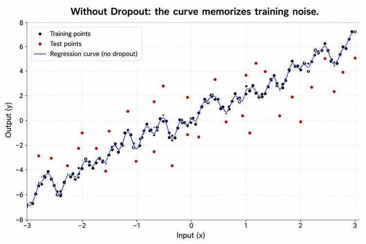
Now we add a single Dropout layer with p = 0.2 after each hidden layer. Everything else is identical, same architecture, same learning rate, same optimizer, same number of epochs.
The training loss goes up slightly with dropout, but the model is no longer perfectly memorizing the training data, and the test loss came down dramatically. That is exactly the trade-off you want.A small sacrifice in training performance for a large gain in generalization.
Dropout with Classification Example
The same pattern appears in classification. Same architecture, 128 neurons per hidden layer, but now the output layer uses sigmoid for binary classification.
Without dropout, the decision boundary is jagged and overcomplex. For every small cluster of outlier points that falls on the wrong side, the model carves out a tiny isolated pocket in the boundary to accommodate it. It is memorizing individual outliers instead of learning where the two classes actually separate.
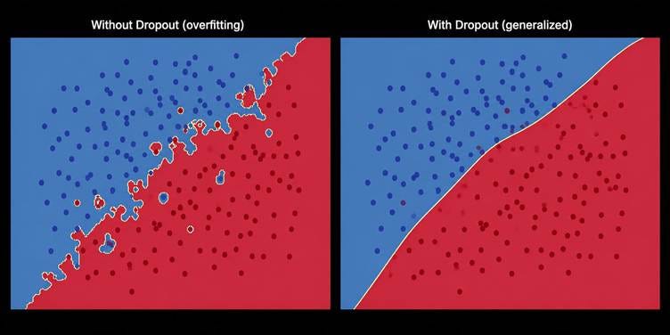
Add dropout at p = 0.5 after each hidden layer and retrain. The boundary smooths out. The model stops chasing outliers and learns the general separation between the two classes instead. Training accuracy drops slightly, but validation accuracy climbs. The model is now actually better on data it has not seen, which is exactly the trade-off you are looking for.
The Effect of p: Finding the Sweet Spot
The dropout rate p is a hyperparameter you need to tune carefully. Too low and you get almost no regularization. Too high and the network cannot learn at all.
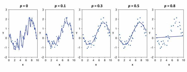
The table below shows what to expect at each range.
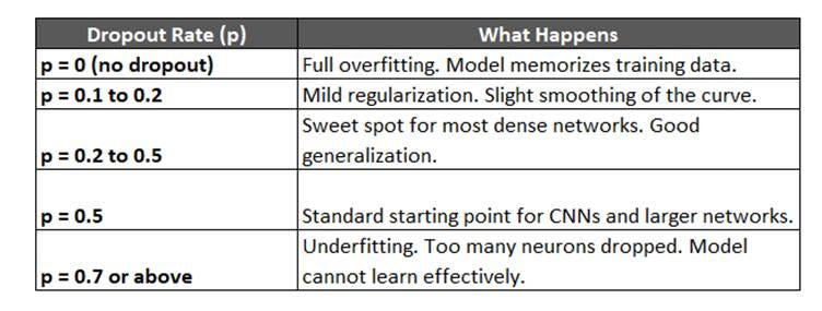
As a rule of thumb, start at p = 0.2. If you see overfitting (training loss much lower than validation), increase p. If you see underfitting (both losses high), decrease p.
Practical Tips for Using Dropout
1. Start with the last hidden layer only
Do not apply dropout to every layer at once. Add it to the last hidden layer first, check if it helps on your validation set, then experiment with adding it to earlier layers.
2. Never apply dropout to the output layer
The output layer must always be fully active. Dropout on the output layer would randomly zero out your predictions, which makes no sense.
3. For CNNs, use lower rates and only on fully connected layers
Convolutional layers have parameter sharing that already provides some regularization. Applying aggressive dropout to convolutional layers is usually counterproductive. If you use dropout on CNN layers, p = 0.2 to 0.3 is more appropriate. Higher rates (0.4 to 0.5) work well on the final fully connected layers of a CNN.
4. For regression vs classification
For regression problems: p between 0.2 and 0.5 tends to work well. For classification: p around 0.5 is a standard starting point for the hidden layers.
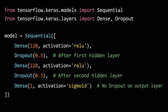
Dropout: Keras Implementation
Downsides of Dropout
1. Slower convergence (experimentally proven)
When neurons are randomly switched off at each training step, the effective learning signal is noisier. The network takes more steps to settle into stable weights. You will typically need more epochs to reach the same training loss. This is a known, documented side effect.
2. The loss function changes every step, making debugging harder
Your optimizer is updating weights based on the gradient of the loss. But with dropout, a different subset of neurons is active on each step, which means the loss function is technically different each time. The gradient calculation becomes harder to interpret.
In practice, this means that if something is going wrong in your network like a bug, a bad layer, or a numerical issue , it is harder to diagnose because the loss curve is noisier and less predictable. This is the biggest downside of dropout.
Regularization
The Problem Regularization Solves: Weights Growing Too Large
Regularization addresses overfitting from a completely different angle than Dropout.
When a neural network overfits, you can often diagnose it by looking directly at the weights. Overfit networks tend to develop very large weight values. This is because large weights allow a neuron to become extremely sensitive to fire very strongly for very specific input patterns that exist only in the training data.
A neuron with a large weight is like a student who has memorized one very specific answer. They can reproduce it perfectly, but ask them anything slightly different and they are lost.
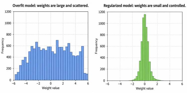
Regularization prevents this by adding a penalty term to the loss function that grows proportionally with the size of the weights. The optimizer, which we covered in the previous article, now has to minimize two things at once that is fit the data well, and keep the weights small.
Total Loss = Original Loss + λ × Penalty Term
Where Original Loss is the task loss your network was already minimizing, such as MSE for regression or Cross-Entropy for classification.
The penalty term is what distinguishes L1 from L2 regularization.
L2 Regularization (Weight Decay)
L2 regularization adds the sum of squared weight values to the loss:
Total Loss = Original Loss + λ × Σ(wⱼ²)
Where the sum is taken over all weights wⱼ in the network
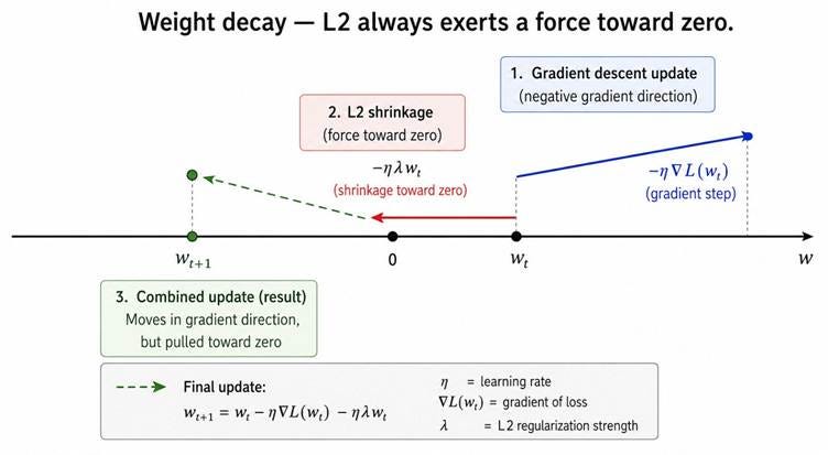
The squaring is significant. A weight of 10 contributes 100 to the penalty. A weight of 1 contributes just 1. Large weights are penalized disproportionately. The optimizer has a strong incentive to reduce large weights, but small weights can survive with little penalty.
The result is that weights shrink toward 0 but never quite reach it. The network still gets to use all its connections, but no single connection can dominate the prediction. L2 is the most common regularization choice for neural networks.
How L2 Affects the Cost Function Shape
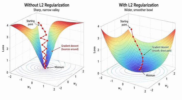
When a network overfits without regularization, the cost function landscape often has a narrow, elongated valley. It fits the training data so specifically that moving away from the exact training-fit weights increases the loss steeply.
L2 regularization smooths this out. The penalty term adds a gentle bowl shape to the loss, making the landscape more uniform. Gradient descent can now converge reliably from many different starting points, not just from carefully chosen ones near the narrow valley.
Notice this connects directly back to what we discussed in Batch Normalization: normalizing inputs makes the cost function landscape more uniform, which helps gradient descent. L2 regularization does something similar, but from the weight side rather than the input side.
L1 Regularization
L1 regularization adds the sum of absolute weight values to the loss:
Total Loss = Original Loss + λ × Σ|wⱼ|
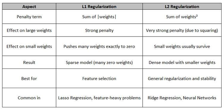
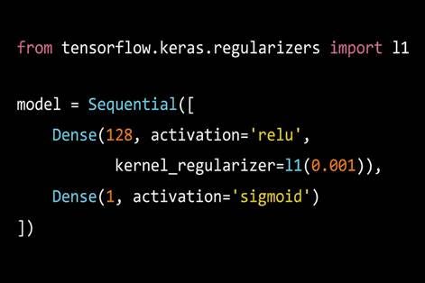
The difference from L2 is in what happens to small weights. The L1 penalty does not taper off as weights get smaller instead, it exerts a constant pressure toward 0 regardless of the weight’s size. This pushes many weights all the way to exactly 0.
When a weight becomes exactly 0, that connection is removed. The network becomes sparse, it uses fewer connections, keeping only the ones it deems most important for the prediction.
L1 is most useful when you believe many of your input features are irrelevant. In that case, you want the network to 0 out the weights for those features. L2 would just shrink them to near-zero, whereas L1 will actually eliminate them.
The choice between L1 and L2 comes down to what you want regularization to do. Here is how they compare.
The Lambda Hyperparameter: Controlling the Trade-off
λ (lambda) is the regularization strength. It controls how strongly the penalty is applied relative to the original loss.
Total Loss = [Original Loss] + λ × [Penalty]
Think of it as a dial that balances two competing goals:
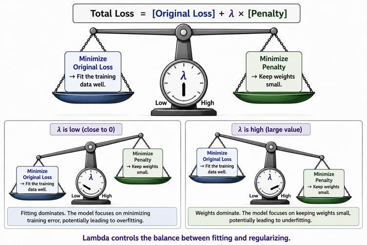
• λ too high: The penalty dominates. Any deviation from 0 is heavily punished. The network cannot build meaningful representations. Therefore underfitting (poor performance on both training and test data).
• λ too low: The penalty barely registers. Weights grow freely. Overfitting returns: great on training data, poor on test data.
• λ just right: The model fits the training data well while keeping weights controlled. Good performance on both training and test data.
Typical starting range:
λ = 0.001 to 0.01 for most dense neural networks. Tune it against your validation loss, just like any other hyperparameter.
Regularization: Keras Implementation
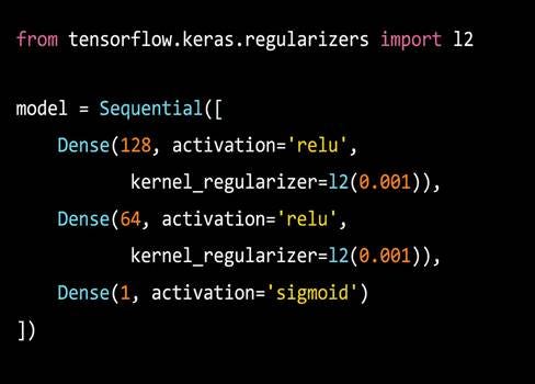
L2 Regularization
L1 Regularization
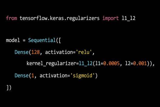
Combined L1 + L2 (Elastic Net)
You can also use both simultaneously . L1 to encourage sparsity and L2 to prevent any single weight from dominating:
Putting It All Together
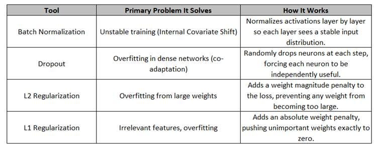
These three tools address different parts of the same problem. Together, they give you a network that trains fast, stays stable, and generalizes.
When to Reach for Each One
Use this as your diagnostic guide:
Training is slow or taking many epochs to converge: use Batch Normalization.
Training is unstable, loss oscillates or diverges: use Batch Normalization.
Training loss is much lower than validation loss: use Dropout, L2 Regularization, or both.
Weights are visibly large: use L2 Regularization.
You suspect many input features are irrelevant: use L1 Regularization.
Sensitive to weight initialization, training varies run-to-run: use Batch Normalization.
Dense (fully connected) network with overfitting: Dropout is your primary regularizer.
CNN with overfitting: Batch Norm on convolution layers, Dropout on fully connected layers.
You want one starting combination that works broadly: Batch Norm + Dropout(0.3) + L2(0.001).
The Intuition to Take Away
Neural networks will overfit. Given enough capacity and time, they memorize rather than learn. These three tools exist to stop that.
Batch Normalization gives each layer a stable distribution to learn from.
Dropout forces each neuron to build independent representations.
Regularization keeps weights from growing too large and too confident.
Use them together. Tune against validation loss and watch the gap close.