
Gradient Boosting for Classification

In my previous article, we explored Gradient Boosting for regression problems. Now, we will dive into how Gradient Boosting works for classification tasks. While the core principles remain the same, additive modeling and sequential learning, classification introduces some important differences, particularly in how we handle probabilities and make predictions
In binary classification, models do not predict class labels or probabilities directly. Instead, they predict real-valued scores in log-odds (logit) space. These scores are then converted into probabilities using the sigmoid function. During training, the predicted probabilities (obtained from the log-odds) are compared with the true labels using the log loss (cross-entropy), and the model parameters are optimized to minimize this loss.
Let’s work with a student admission dataset to understand the Gradient Boosting algorithm. Consider data from a university admission process:
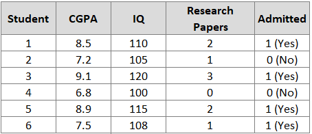
Input Features (X): CGPA, IQ, Research Papers
Target (y): Admission status (0 = Not Admitted, 1 = Admitted)
Goal: Predict probability of admission for new students
In this example:
4 students were admitted (y = 1)
2 students were not admitted (y = 0)
Total: 6 observations
Understanding Log(Odds)
Odds represent the ratio of the probability of success to the probability of failure:
Where p is the probability of the positive class (being admitted).
Examples:
If p = 0.5: Odds = 0.5/0.5 = 1 (even odds)
If p = 0.8: Odds = 0.8/0.2 = 4 (4:1 in favor of admission)
If p = 0.2: Odds = 0.2/0.8 = 0.25 (4:1 against admission)
Log(Odds) is the natural logarithm of the odds:
This is also called the logit function.
Conversely, Probability from Log(Odds):
Or equivalently:
This is the sigmoid function or logistic function.
Why Log(Odds) Space Works Better in Gradient Boosting
In gradient boosting for classification, we work in log(odds) space rather than probability space for the following reasons:
1. Unconstrained Prediction Space
Probabilities are constrained between 0 and 1. Log(odds) ranges from -∞ to +∞. Iterative corrections are easier in unconstrained space since predictions never go out of bounds.
2. Better Gradients
Gradients guide new tree additions. In probability space, gradients shrink near 0 or 1, slowing learning. Log(odds) space keeps gradients well-behaved with better magnitudes.
3. Mathematical Convenience
Log loss derivatives produce clean expressions in log(odds) space. The math for optimization is easier.
Algorithm: Step-by-Step
Required Inputs
Training Data: {(xᵢ, yᵢ)}ᵢ₌₁ⁿ where yᵢ ∈ {0, 1}
Loss Function: Log Loss (Binary Cross-Entropy)
Number of Iterations: M (hyperparameter)
The Loss Function
For binary classification, we use Log Loss:
Where:
y = actual label (0 or 1)
p = predicted probability
F(x) = log(odds) = log(p / (1 - p))
This can be rewritten in terms of F(x):
This form is more convenient for computing derivatives.
Step 0: Understanding the Geometric Intuition
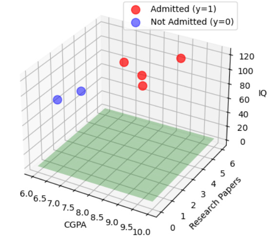
Imagine plotting data in feature space: admitted students (y=1) as red dots, non-admitted (y=0) as blue dots. Gradient boosting iteratively builds the decision boundary to separate them. It starts from baseline log(odds), fits trees to residuals, and updates until high-CGPA/high-research points land on the admitted side while low-CGPA/low-research points stay on the non-admitted side.
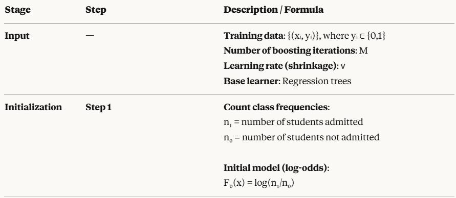
Step 1: Initialize the Model - Finding F₀(x)
Just like in regression, we start with an initial prediction:
For binary classification with log loss, the loss is L(y,F(x))=log(1+e^F(x))−y⋅F(x).
The initial prediction F₀(x)=γ is the constant value that minimizes this loss across all training examples. This γ becomes our baseline F₀(x), typically log(ȳ/1−ȳ) for proportion ȳ of positive cases.
Mathematical Derivation
To find the minimum, take the derivative with respect to γ and set it to zero:
Loss function (average log loss)
Take derivative with respect to γ
Set derivative equal to zero
Define empirical mean of labels
Substituting we get:
rerranging the above terms and solving for γ we get
Final result (log-odds form)
Let the training set contain ( n ) samples, with binary labels yᵢ(0,1)
Empirical mean of the labels is:
Since yᵢ∈{0,1} ,where yᵢ=1 for admitted (positive) examples and yᵢ=0 for non-admitted (negative) examples, the sum ∑yᵢ simply counts the total number of positive examples n₁ in our dataset, while n₀=n−n₁ counts the negative examples
Thus, the empirical positive class probability is:
The initial probability is the proportion of positive examples in the training data!
The initial prediction F₀(x) in gradient boosting classification is the log-odds of the class proportion, Substituting into the expression for the initial model:
They are the same quantity, just written from:
a probability viewpoint p
a data-averaging viewpoint ȳ
From our dataset:
4 students admitted (y=1) → n₁ = 4
2 students not admitted (y=0) → n₀ = 2
Therefore:
p = 4/6 = 0.667 (66.7% of students were admitted)
F₀(x) = log(4/2) = log(2) ≈ 0.693
This log(odds) value of 0.693 becomes our initial prediction for all students.
To verify converting back to probability:
This makes intuitive sense because without knowing anything about a student’s CGPA, IQ, or research papers, our best guess is that they have a 66.7% chance of admission (the overall admission rate).
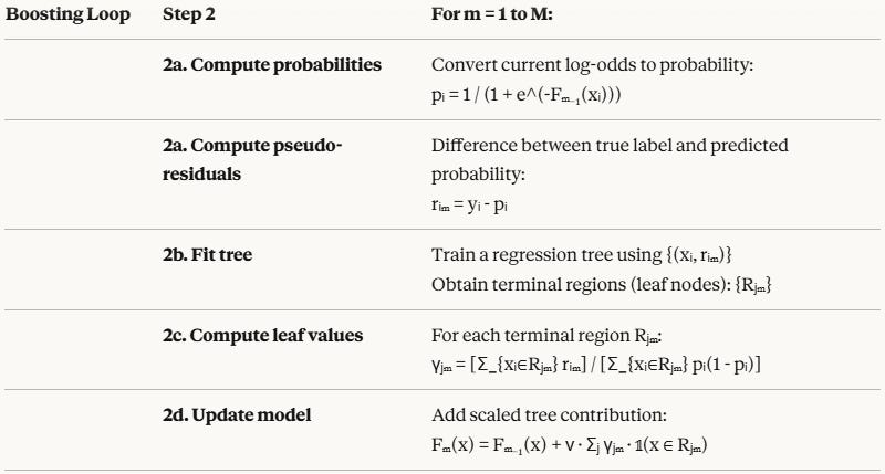
Step 2: The Iterative Process
Now we enter the main loop (repeat M times).
Step 2.1: Compute Pseudo-Residuals
For each observation i, calculate:
This is the negative gradient of the loss function.
Mathematical Derivation
Starting with the log loss:
Taking the derivative with respect to F:
Recall that e^F / (1 + e^F) = p (the sigmoid of F), so:
Therefore, the pseudo-residual is:
Where:
yᵢ = actual label (0 or 1)
pᵢ = current predicted probability =
\(\frac{1}{1 + e^{-F_{m-1}(x_i)}} \)
Interpretation: The pseudo-residual is the difference between the actual label and predicted probability.
If student was admitted (y=1) and p=0.6: residual = 0.4 (prediction too low, increase log(odds))
If student was not admitted (y=0) and p=0.3: residual = -0.3 (prediction too high, decrease log(odds))
If student was admitted (y=1) and p=0.9: residual = 0.1 (prediction close, small adjustment)
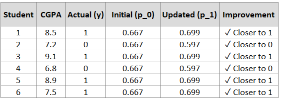
Example Calculation (First Iteration, m=1)
We start with F₀(x) = 0.693 for all students, which gives:
Now compute residuals for each student:
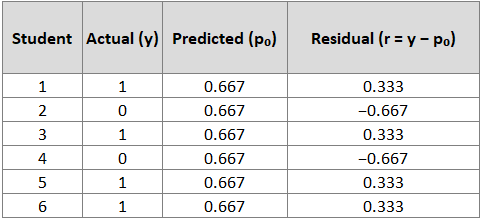
Interpretation:
Students 1, 3, 5, 6 (admitted): Positive residuals (0.333) indicate we need to increase their predicted probability
Students 2, 4 (not admitted): Negative residuals (-0.667) indicate we need to decrease their predicted probability
These residuals tell us how to adjust our predictions to reduce error.
Step 2.2: Fit a Regression Tree
Now fit a regression tree to predict these pseudo-residuals:
Input: Original features (CGPA, IQ, Research Papers)
Target: Pseudo-residuals (r)
Even though we’re solving a classification problem, we fit a regression tree because the pseudo-residuals are continuous values (ranging from -1 to +1).
The tree partitions the data into regions (terminal nodes/leaves). With a simple tree (max_depth=1), we get a decision stump with 2 regions.
Example: First Tree Split
Suppose the tree splits on CGPA < 7.5:
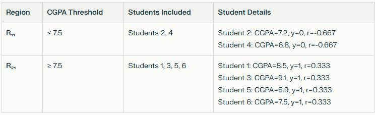
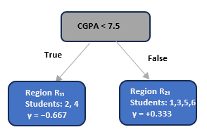
Notice how the tree naturally separates:
Low CGPA students (not admitted) → negative residuals
High CGPA students (admitted) → positive residuals
Step 2.3: Compute Leaf Node Outputs (γⱼₘ)
For each terminal region Rⱼₘ, we compute:
Substituting the log loss:
Mathematical Derivation
Taking the derivative with respect to γ:
This simplifies to:
Let
Then:
Problem: This equation cannot be solved analytically for γ!
Since we can’t solve it directly, we use the Newton-Raphson method to approximate γ.
The Newton-Raphson formula gives:
Where:
rᵢₘ = yᵢ - pᵢ (the pseudo-residual)
pᵢ = current predicted probability for observation i
Intuitive Interpretation:
Numerator: Sum of residuals in the leaf (how much total correction is needed)
Denominator: Sum of p(1-p) values (a weighting term that accounts for prediction confidence)
The term p(1-p) is maximized when p=0.5 (maximum uncertainty) and approaches zero when p is near 0 or 1 (high certainty). This means:
Predictions with high uncertainty get larger adjustments
Predictions with high certainty get smaller adjustments
Example Calculation for Our Student Data
Recall: F₀(x) = 0.693, so p₀ = 0.667 for all students
For Region R₁₁ (Students 2, 4 - low CGPA, not admitted):
Numerator = Sum of residuals:
r₂₁ + r₄₁ = (-0.667) + (-0.667) = -1.334
Denominator = Sum of p(1-p):
[0.667 × 0.333] + [0.667 × 0.333]
0.222 + 0.222 = 0.444
Therefore: γ₁₁ = -1.334 / 0.444 = -3.00
For Region R₂₁ (Students 1, 3, 5, 6 - high CGPA, admitted):
Numerator = Sum of residuals:
r₁₁ + r₃₁ + r₅₁ + r₆₁ = 0.333 + 0.333 + 0.333 + 0.333 = 1.332
Denominator = Sum of p(1-p):
4 × [0.667 × 0.333] = 4 × 0.222 = 0.888
Therefore: γ₂₁ = 1.332 / 0.888 = 1.50
Interpretation:
γ₁₁ = -3.00: For low CGPA students, decrease log(odds) by 3.00 (reduce admission probability)
γ₂₁ = 1.50: For high CGPA students, increase log(odds) by 1.50 (increase admission probability)
These are significant adjustments in the log(odds) space!
Step 2.4: Update the Model
Update the prediction function:
Fₘ(x) = Fₘ₋₁(x) + ν · Σⱼ γⱼₘ · I(x ∈ Rⱼₘ)
Where:
ν is the learning rate (typically 0.1)
I(x ∈ Rⱼₘ) is an indicator function (1 if x is in region Rⱼₘ, 0 otherwise)
Simplified: Fₘ(x) = Fₘ₋₁(x) + ν · hₘ(x)
Where hₘ(x) is the tree’s output for observation x.
Example: After First Iteration (with ν = 0.1)
For students in R₁₁ (low CGPA - Students 2, 4):
F₁(x) = F₀(x) + 0.1 × γ₁₁
F₁(x) = 0.693 + 0.1 × (-3.00)
F₁(x) = 0.393
Converting to probability:
For students in R₂₁ (high CGPA - Students 1, 3, 5, 6):
F₁(x) = F₀(x) + 0.1 × γ₂₁
F₁(x) = 0.693 + 0.1 × (1.50)
F₁(x) = 0.843
Converting to probability:
Summary of improvements:
After just one iteration, all predictions have moved in the right direction!
Step 2 Repeated: Second Iteration (m=2)
We now repeat the process with updated predictions.
Step 2.1: Compute New Pseudo-Residuals
Using p₁ values from the previous iteration:
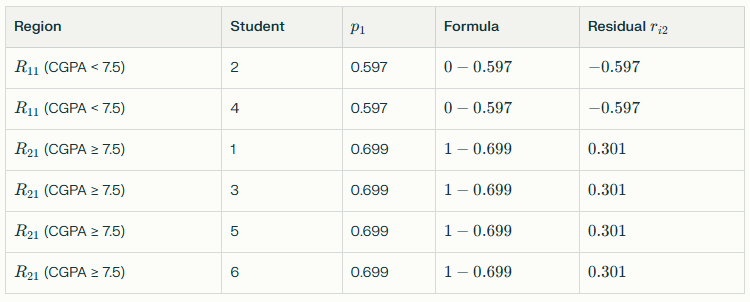
Notice the residuals are smaller than before.
Step 2.2-2.4: Fit Tree, Compute γ, Update Model
The second tree might split on a different feature like Research Papers < 2 to further refine the decision boundary, separating high-CGPA students with few papers (lowering their probabilities) from those with many papers (increasing theirs).
This process continues for M iterations, each time computing residuals from the current predictions, fitting a tree to capture remaining patterns, computing optimal leaf values using Newton-Raphson, and updating the model with a small step controlled by the learning rate.
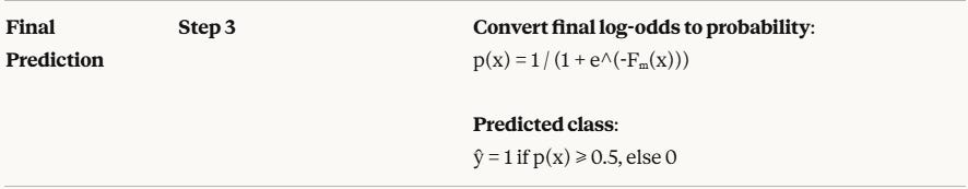
Step 3: Making Final Predictions
After M iterations, we have the final model:
F(x) = F₀(x) + ν·[h₁(x) + h₂(x) + ... + hₘ(x)]
This gives us log(odds). To get probabilities:
p(x) = 1 / (1 + e^(-F(x)))
To get class predictions:
If p(x) ≥ 0.5: Predict class 1 (Admitted)
If p(x) < 0.5: Predict class 0 (Not Admitted)
Predicting for a new datapoint
CGPA = 8.0 ,IQ = 112 , Research Papers = 2
The model evaluates:
Initial prediction: F₀ = 0.693 (baseline log(odds))
Tree 1 (CGPA split): Student has CGPA ≥ 7.5 → adds 0.15 → F = 0.843
Tree 2 (Research split): Student has Papers ≥ 2 → adds 0.08 → F = 0.923
Tree 3 (IQ split): Student has IQ ≥ 110 → adds 0.05 → F = 0.973
... continue for M trees ...
After M=50 iterations, suppose F(x) = 1.8 for this student:
Prediction: Admitted (class 1) with 85.8% confidence
The algorithm evolved from a simple baseline based on the overall admission rate (66.7%) to a sophisticated classifier by first using CGPA to separate high and low performers, then progressively incorporating research papers, IQ scores, and their interactions, ultimately combining all trees to produce well-calibrated probabilities for nuanced admission decisions.
Complete Algorithm Summary
Why This Approach Works
1. Additive Model in Log-Odds Space
Gradient boosting builds the prediction function (F(x)) as a sum of many small trees. Working in log-odds space allows unrestricted positive and negative updates, which is not possible in probability space where values must stay between 0 and 1.
2. Gradient Descent in Function Space
Instead of optimizing parameters directly, each tree is trained to fit the negative gradient of the loss function with respect to the current model. This guarantees that every iteration reduces the overall loss.
3. Sequential Error Correction
Each new tree focuses on correcting mistakes made by previous trees. Students who were admitted but predicted with low probability receive positive corrections, while non-admitted students predicted with high probability receive negative corrections.
4. Probabilistic Framework
The final model output in log-odds space is converted to probabilities using the sigmoid function. This produces well-calibrated probabilities that can be used for ranking candidates, setting flexible decision thresholds, and understanding model confidence.
5. Ability to Handle Complex Patterns
Decision trees allow gradient boosting to capture non-linear relationships, feature interactions (such as CGPA combined with research experience)
6. Adaptive Learning Behavior
The Newton–Raphson update automatically adjusts step sizes: larger updates are made when predictions are uncertain (probabilities near 0.5), and smaller updates are made when predictions are already confident (probabilities near 0 or 1).
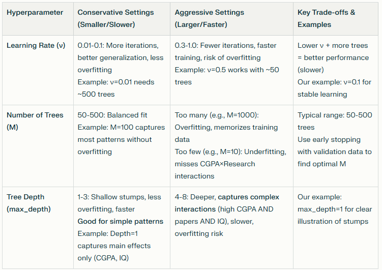
Practical Considerations
The table below highlights practical considerations in gradient boosting such as controlling training speed, managing model complexity, balancing bias–variance trade-offs, preventing overfitting and choosing stable hyperparameter values in real-world applications.
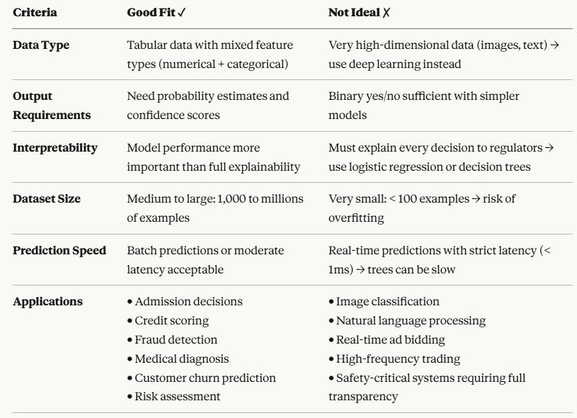
When to Use Gradient Boosting for Classification
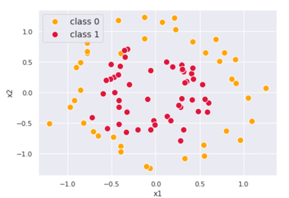
Common Pitfalls and How to Avoid Them
This table summarizes common mistakes and best practices, showing the correct way to handle key concepts and why they matter in practice.
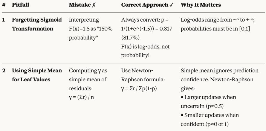
Visual Intuition
To build deeper intuition, let’s visualize the process in 3D space with simple data (two features x₁ and x₂, binary class y).
Initial Prediction Plane
The first prediction is a flat plane at height p = mean(y).
")
In a sample dataset where mean(y) = 0.56, everything is initially classified as class 1.
Visualizing Residuals
Residuals appear as vertical lines from each point to the prediction plane.
")
After First Tree
The first tree creates a step-like surface, improving predictions in different regions.
Here we are creating the first tree predicting the residuals with two different values r = {0.1, -0.6}.
")
Each boosting step updates predictions additively in log-odds space using scaled γ values, and when transformed back to probability space, these updates form a characteristic stair-shaped prediction curve, illustrated in the next figure.
If we convert log-odds F(x) back into the predicted probability p(x), it looks like a stair-like object below.
")
The purple-colored plane is the initial prediction p₀ and it is updated to the red and yellow plane p₁.
Now, the updated residuals r look like this:
")
Second Iteration
In the next step, we create a regression tree again using the same x₁ and x₂ as features and the updated residuals r as its target. Here is the created tree:
")
We apply the same formula to compute γ and update prediction F₂(x)
Again, if we convert log-odds F₂(x) back into the predicted probability p₂(x), it looks like something below.
")
The Iterative Process
We iterate these steps until the model prediction stops improving. The figures below show the optimization process from 0 to 4 iterations.
")
You can see the combined prediction p(x) (red and yellow plane) is getting closer to our target y as we add more trees into the combined model. This is how gradient boosting works to predict complex targets by combining multiple weak models.
Flowchart of complete algorithm process - Initialize → Compute Residuals → Fit Tree → Compute Gamma → Update Prediction → Repeat
Conclusion
Gradient Boosting for classification extends the regression framework by operating in log-odds space, using log loss for probabilistic predictions, computing leaf values via Newton-Raphson, and applying sigmoid for final outputs. It is powered by five core strengths:
Sequential Error Correction: Each tree systematically addresses residuals left by predecessors
Flexible Decision Boundaries: Captures complex rules like “high CGPA OR (moderate CGPA AND many papers)”
Probabilistic Predictions: Sigmoid provides confidence levels, not binary decisions
Gradient-Based Optimization: Mathematically guaranteed improvement per iteration
Adaptive Step Sizes: Newton-Raphson auto-adjusts based on prediction confidence
Practical Impact: Real-world applications gain sequential error correction (each tree fixes predecessors’ mistakes), better decisions for borderline cases, consistent fairness across applicants, transparency via feature importance (key predictors ranked), and efficient automation for thousands of applications.
This comprehensive guide covered the complete mathematical derivation of gradient boosting for binary classification. The same principles extend to multi-class classification (e.g., predicting which of 5 academic programs a student should join) using the softmax function and categorical cross-entropy loss.